1 Introduction
Expected Threat (xT) is a discrete time Markov chain model that measures the probability of a goal being scored from a particular zone of a pitch. The pitch is usually split in 16 by 12 (length x width), resulting in 192 available zones. Once the pitch is split, you can calculate the xT of given zone by the following formula:
\[xT_{x, y} = (s_{x, y} \times g_{x, y}) + (m_{x, y} \times \sum_{l=1}^{16} \sum_{w=1}^{12} T_{(x, y)} \rightarrow _{(l, w)}xT_{l,w})\]\(s_{x, y}\) is the probability of taking a shot from particular zone. \(m_{x, y}\) is the probability of player move from particular zone via dribble or pass. Since the xT model assumes players can only move or shoot given the location, \(s_{x, y} + m_{x, y} = 1.\)
Finally, \(g_{x, y}\) is the probability of goals being scored from particular zone. \(\sum_{l=1}^{16} \sum_{w=1}^{12} T_{(x, y)} \rightarrow _{(l, w)}xT_{l,w}\) is the probability of moving from one particular zone to all other zones including itself, multiplied by the values of these zones.
Initially, \(xT_{l,w}\) is set to 0, and iterate n times until convergence, meaning the probability of a goal scored in the next n actions.
This way, we can calculate cumulative xT for all actions performed by each player, compare the value among other players to evaluate individual performance. Or we can calculate xT per team to see where the team creates scoring opportunities.
2 Data
The data used in this project is Statsbomb open data.
- The data is available at the Statsbomb github page
- User agreement can be found here
- Competitions provided in the free data can be found here
This project used the World Cup 2022 data which is provided in nested JSON-format. Some pre-processing are required before calculating Expected Threat.
First, we need to get competition_id and season_id of our data of interest. According to the competition document, competition_id and season_id for WC 2022 are 43 and 106 respectively. We can now grab all match_ids in the competition by following:
competition_id = 43
season_id = 106

file_path = os.path.join("..", "..", "data", "statsbomb_raw_data", "matches", str(competition_id), str(season_id) + ".json")

with open(file_path, "r", encoding='utf-8') as f:
    match_data = json.load(f)

match_ids = [match['match_id'] for match in match_data]
Now we can grab all event data of interest, create a pandas dataframe with the obtained match_ids.
data_dir = '../../data/statsbomb_raw_data/events'
event_list = []

for match_id in match_ids:

    away_team_name = get_away_team_name(match_id, match_data)

    file_path = os.path.join(data_dir, f"{match_id}.json")

    with open(file_path, 'r', encoding='utf-8') as f:
        events = json.load(f)

    for event in events:

        if event['type']['name'] in ['Shot', 'Pass', 'Carry']:
            data = {
                'event_id': event['id'],
                'event_type': event['type']['name'],
                'team_against': away_team_name,
                'minute': event['minute'],
                'second': event['second'],
                'player_id': event['player']['id'],
                'player_name': event['player']['name'],
                'x_start': event['location'][0],
                'y_start': event['location'][1],
                'x_end': None,
                'y_end': None,
                'pass_length': None,
                'pass_type': None,
                'outcome': 0
            }

            if event['type']['name'] == 'Carry':
                data['x_end'] = event['carry']['end_location'][0]
                data['y_end'] = event['carry']['end_location'][1]
                data['outcome'] = 1

            elif event['type']['name'] == 'Pass':
                data['x_end'] = event['pass']['end_location'][0]
                data['y_end'] = event['pass']['end_location'][1]
                data['outcome'] = 1 if 'outcome' not in event['pass'] else 0
                data['pass_length'] = event['pass']['length']
                data['pass_type'] = event['pass']['height']['name']

            elif event['type']['name'] == 'Shot':
                data['outcome'] = 1 if event['shot']['outcome']['name'] == 'Goal' else 0
            event_list.append(data)
df = pd.DataFrame(event_list)
Now that the data comes in a clean and tabular format, let’s call this event_data and this is the primary dataset to calculate xT. Some of the key features of event_data include:
- event_type: The type of action performed by a player, such as a dribble, pass, or shot.
- player_id: A unique identifier assigned to each player.
- player_name: The name of the player associated with the action.
- x_start: The starting x-coordinate of the action on the pitch.
- y_start: The starting y-coordinate of the action on the pitch.
- x_end: The ending x-coordinate of the action on the pitch.
- y_end: The ending y-coordinate of the action on the pitch.
- outcome: The result of the action, 1 = successful and 0 otherwise.
All the probabilities and matrix can be calculated from this dataset. We now seem ready and go ahead to calculate xT, but there is one additional preprocessing step required: determining the total play time for each player. This is crucial because players’ play times can vary significantly, with some participating in over 400 minutes of play and others only exceeding 90 minutes.
Play time is stored in open-data/data/lineups. For each game, there is a nested JSON data. Within the JSON file, there are fields such as player_id, player_name, from, and to, which represent the player’s unique identifier, their name, and the time range (in minutes) during which they were on the pitch. We can calculate the difference between to and from to get the total play time per game, repeat this process for all 64 games in WC.
player_dict = {}

for match_id in match_ids:
    file_path = os.path.join(data_dir, f"{match_id}.json")

    with open(file_path, 'r', encoding='utf-8') as f:
        player_data = json.load(f)

    for x in player_data:
        for player_info in x['lineup']:
            player_id = player_info['player_id']
            player_name = player_info['player_nickname'] if player_info['player_nickname'] else player_info['player_name']
            country = player_info['country']['name']

            if player_id not in player_dict:
                player_dict[player_id] = {
                    'player_name': player_name,
                    'country': country,
                    'total_play_time': 0,
                }
            if len(player_info['positions']) > 0:
                total_time = 0
                for i in range(0, len(player_info['positions'])):
                    from_time = to_minutes(player_info['positions'][i]['from'])
                    to_time = to_minutes(player_info['positions'][i]['to']) if player_info['positions'][i]['to'] else 90
                    total_time += (to_time - from_time)

                player_dict[player_id]['total_play_time'] += total_time
This new dataframe player_data has the following features:
- player_id: A unique identifier assigned to each player.
- player_name: The name of the player.
- country: The name of the country associated with the player.
- total_play_time: The total amount of time the player has played during the world cup 2022.
3 Implementation
Data is now ready for further analysis, we can start calculating xT by first splitting the pitch into 192 grids (12 width x 16 length).
class XTModel:
    def __init__(self, w=12, l=16):
        self.width = w
        self.length = l
        self.pitch_length = 120
        self.pitch_width = 80

    def get_zone(self, x, y):

        if np.isnan(x) or np.isnan(y):
            return np.nan, np.nan

        zone_length, zone_width = self.pitch_length / self.length, self.pitch_width / self.width

        zone_x = int(x // zone_length)
        zone_y = int(y // zone_width)

        if zone_x == self.length:
            zone_x -= 1
        if zone_y == self.width:
            zone_y -= 1

        return zone_x, zone_y
Here we define the class XTModel, we can use a method get_zone to split the pitch. It calculates the size of each zone by dividing the pitch dimensions by the number of zones in each direction. It then calculates the zone indices for the given x and y coordinates. If the calculated indices are equal to the number of zones in their respective directions, they are decremented by 1 to ensure they fall within the grid’s bounds.
def calculate_matrix(self, df):
    df[['zone_start_x', 'zone_start_y']] = df.apply(lambda row: pd.Series(self.get_zone(row['x_start'], row['y_start'])), axis=1)
    df[['zone_end_x', 'zone_end_y']] = df.apply(lambda row: pd.Series(self.get_zone(row['x_end'], row['y_end'])), axis=1)

    move_matrix = np.zeros((self.width, self.length))
    shot_matrix = np.zeros((self.width, self.length))
    goal_matrix = np.zeros((self.width, self.length))

    for _, row in df[df['event_type']!='Shot'].iterrows():
        zone_x, zone_y = row['zone_start_x'], row['zone_start_y']
        move_matrix[zone_y, zone_x] += 1

    for _, row in df[df['event_type']=='Shot'].iterrows():
        zone_x, zone_y = row['zone_start_x'], row['zone_start_y']
        shot_matrix[zone_y, zone_x] += 1

        if row['outcome'] == 1:
            goal_matrix[zone_y, zone_x] += 1

    total_matrix = move_matrix + shot_matrix

    score_matrix = np.divide(goal_matrix, shot_matrix, where=shot_matrix!=0)

    move_matrix = np.divide(move_matrix, total_matrix, where=total_matrix!=0)

    shot_matrix = np.divide(shot_matrix, total_matrix, where=total_matrix!=0)

    return move_matrix, shot_matrix, score_matrix
We can now call calculate_matrix to get the matrices. The move_matrix and shot_matrix are generated by counting the number of times a player chooses to move or take a shot for each grid cell. By summing these two matrices, we can compute the total_matrix. We can then divide both move_matrix and shot_matrix by total_matrix. This gives us the probability distribution of moves and shots for each grid cell on the field.
def calculate_transition_matrix(self, df):
    success_moves = df[df['event_type'].isin(['Pass', 'Carry']) & df['outcome']==1]

    X = pd.DataFrame()
    X['start_x'] = success_moves['zone_start_y'] * (self.length) + success_moves['zone_start_x']
    X['end_x'] = success_moves['zone_end_y'] * (self.length) + success_moves['zone_end_x']
    X['end_x'] = X['end_x'].astype(int)

    start_zone_counts = X['start_x'].value_counts(sort=False)

    start_zone_total_counts = np.zeros(self.length*self.width)

    start_zone_total_counts[start_zone_counts.index] = start_zone_counts

    transition_matrix = np.zeros((self.width*self.length, self.width * self.length))

    for i in range(0, self.width*self.length):
        end_zone_counts = X[X['start_x']==i]['end_x'].value_counts(sort=False)
        transition_matrix[i, end_zone_counts.index] = end_zone_counts / start_zone_total_counts[i]

    return transition_matrix
The final step is to calculate transition_matrix, which is a matrix representing the probabilities of successfully transitioning from one grid zone to any other grid zone.
The matrix has dimensions (192, 192). Each row i in the matrix corresponds to a starting grid zone, and each column j corresponds to an ending grid zone. The value transition_matrix[i, j] represents the probability of a successful transition from grid zone i to grid zone j.
We can finally plug all the matrices obtained in the equation (1) to calculate xT for all the grids.
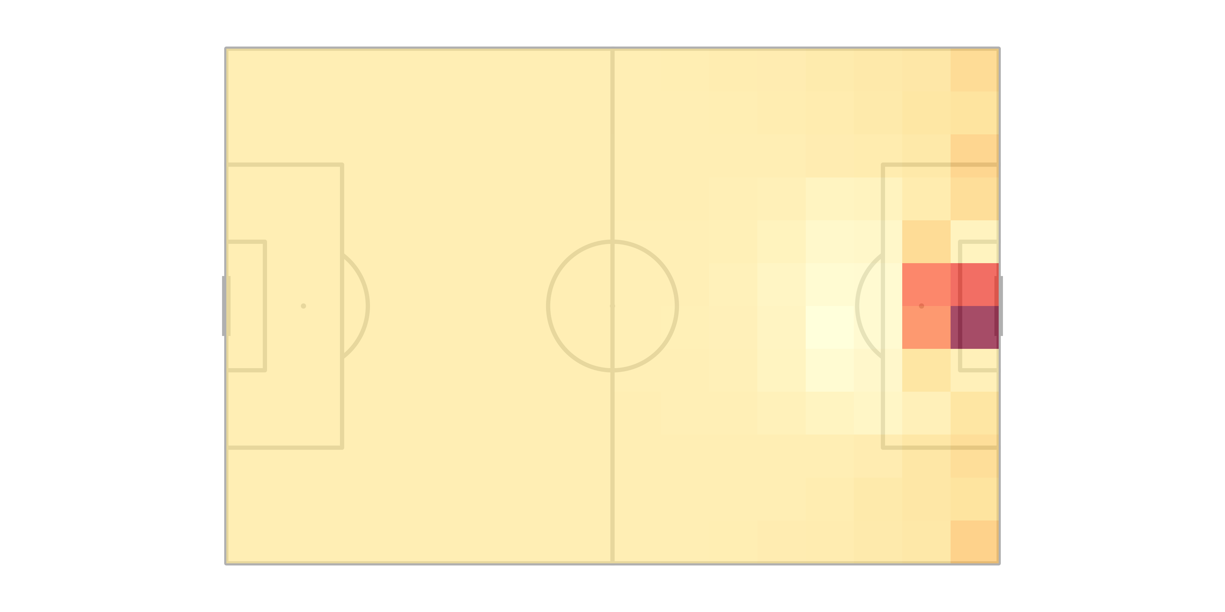
The plot above displays the xT values for each grid zone. In general, the closer a zone is to the goal, the more likely a team is to score within the next few actions. One interesting insight from the plot is that the area immediately outside the penalty area, previously known as Zone 14, has a lower likelihood of scoring. This zone was once believed to be vital for successful teams due to the multiple attacking options it provided. However, it seems that teams have developed effective defensive tactics to counter the offensive advantages of this zone. This makes sense, as teams usually have limited preparation time before the World Cup; they may prioritize certain areas of the field to defend more effectively.
4 Calculating xT for All Actions
Based on the xT grids obtained, we can now assign a xT value to each successful action during the WC. we can simply calculate the difference between xt value of starting grid and xT value of ending grid to calculate the xt value for the action.
For example, let’s examine Kaoru Mitoma’s two successful actions in the clip. We will focus on his first action, where he carries the ball from near the sideline into the penalty box. To calculate the Expected Threat (xT) for this action, we can follow these steps:
\[xT_{\text{carry}} = xT_{\text{end}} - xT_{\text{start}} = 0.169607 - 0.157658 = 0.011949\]xT for his subsequent cutback is calculated as follows:
\[xT_{\text{pass}} = xT_{\text{end}} - xT_{\text{start}} = 0.282051 - 0.169607 = 0.112445\]This indicates his series of actions produced over 12% of probability of scoring in the next few actions.
We can repeat this process for all actions, and then group by each player to get individual statistics.
5 Visualisation
5.1 Individual Performance
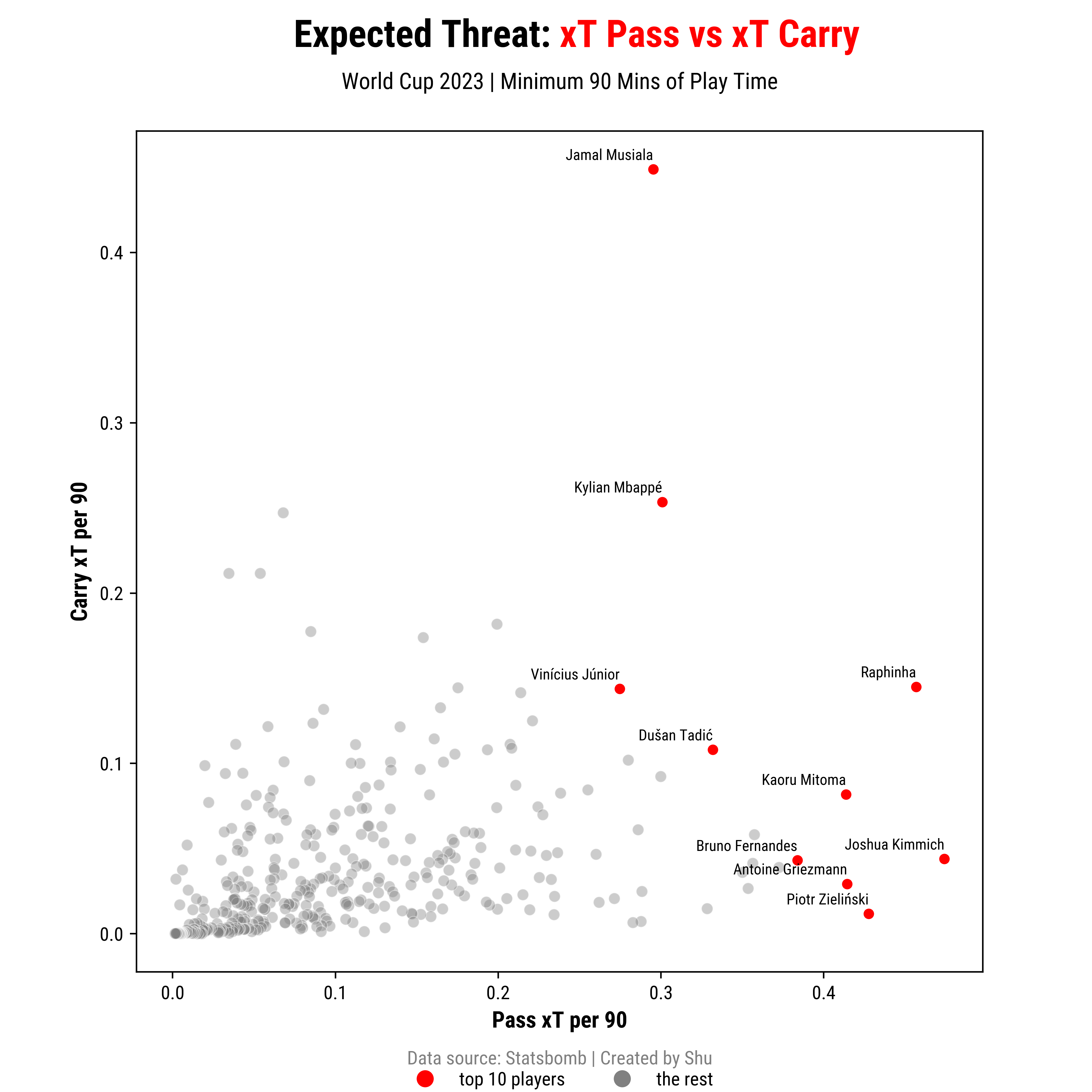
The figure shows the Expected Threat (xT) per player, which was normalised per 90 mins. It also shows the contribution of xT from both passes and carries. From the plot, one can see a noticeable trend: a larger proportion of xT is generated through passes rather than carries. This observation is indicative of the defensive playing styles adopted by teams during the World Cup, which restricted space in advantageous areas for dribblers to exploit. Nonetheless, one striking outlier warrants attention — Jamal Musiala, who remarkably produced over 0.4 xT per 90 minutes through carries alone. This extraordinary performance distinguishes Musiala from his peers and highlights his exceptional ability to create goal-scoring opportunities through carries.
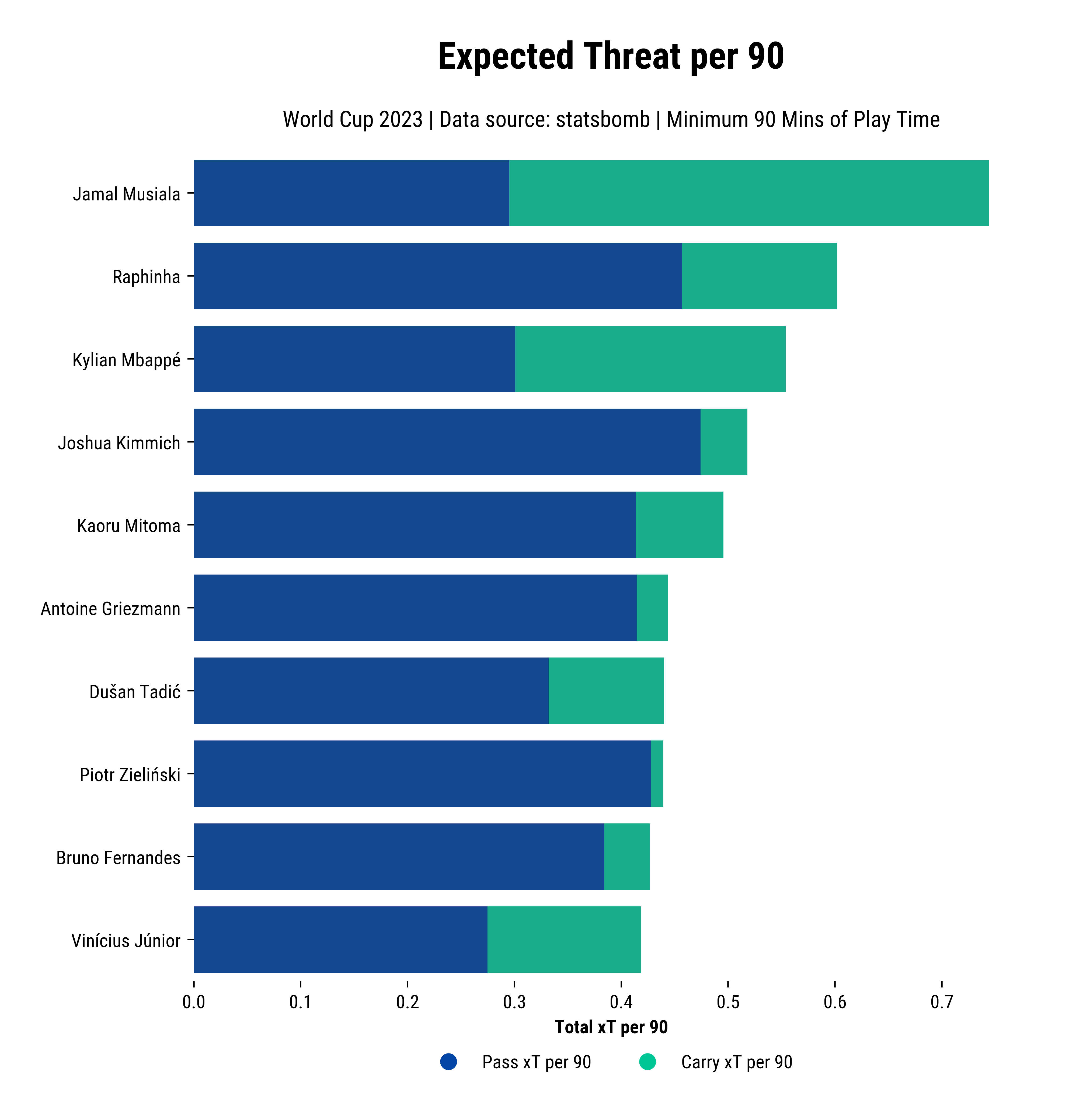
I have also created a bar graph to illustrate the contribution of pass and carry to xT. Musiala, Mbappé, and Vinícius emerged as the top 3 dribblers in terms of carry xT, while Kimmich, Raphina, and Zieliński led in creating chances through passes.
5.2 Team Performance
Finally, xT can also be used to evaluate team’s tactical behaviour. That is, where do teams create the most chances from?
To answer this question, we can calculate xT grids per team/country. This could be helpful determining the opponent’s style of play/tactics.

The above plot shows xT calculated per team basis, It is evident that certain teams exhibit preferences for specific areas when in possession.
6 Conclusion
In this project, I went over a simple implementation of Expected Threat in python using Statsbomb open data. It was an excellent learning opportunity to understand one of the advanced football metrics today. All resource for completing this project are following:
- Karun Singh’s blog post on Expected Threat
- Abhishek Sharma’s blog post on Expected Threat
- Socceraction by KU Leuven: Implementation of Expected Threat in Python
- David Sumpter’s article on Expected Threat: For understanding its mathematical concept
- Soccerment.com: for inspirational data viz